NL1333DBAE1S-ES Datasheet: Complete Specs & Pinout Guide
The NL1333DBAE1S-ES is a low‑power, rail‑to‑rail input/output operational amplifier that operates from ≈2.1 V, draws only ~17 μA quiescent current, achieves 106 dB CMRR, and exhibits ≈60 nV/√Hz input noise density, making it attractive for portable sensor front ends and battery‑powered data acquisition. This NL1333DBAE1S-ES datasheet guide breaks down core specs, pinout, PCB/layout tips, performance plots to reproduce, and quick application examples so designers can decide fast whether to prototype with this part.
1 — Product overview & key features (Background)
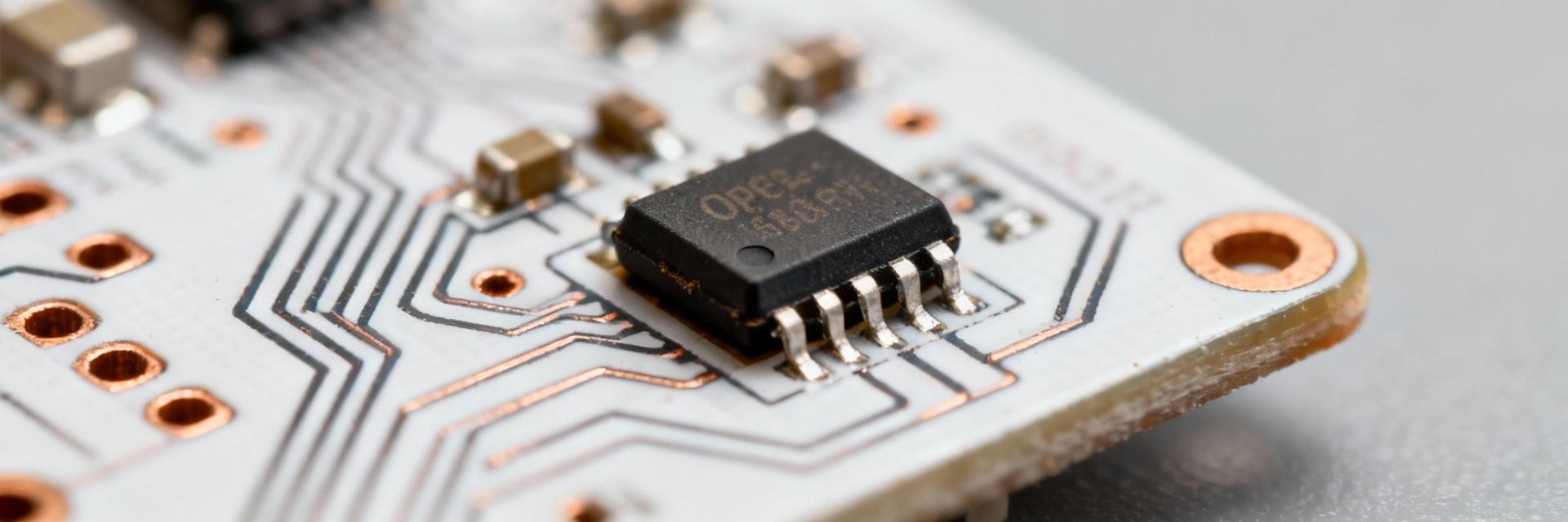
Key features at a glance — what to include
- Supply voltage range: ~2.1 V to 5.5 V — why it matters: supports single‑cell battery systems and low‑voltage digital rails for compact designs.
- Quiescent current: ~17 μA typ — why it matters: extends battery life in always‑on sensing applications.
- Rail‑to‑rail input/output — why it matters: maximizes dynamic range on low supply voltages without level shifters.
- Noise density: ≈60 nV/√Hz and CMRR: 106 dB — why it matters: yields accurate small‑signal amplification in noisy environments.
- Package: small surface‑mount package with thermal pad — why it matters: space‑constrained PCB designs benefit from compact footprints and thermal relief.
Fast takeaway: the NL1333DBAE1S-ES is optimized where ultra‑low quiescent current and good DC accuracy outweigh very high bandwidth, making it ideal when battery life and noise floor dominate selection criteria.
Typical applications & market fit — what to include
Common use cases include portable sensor front‑ends, low‑power data acquisition, battery monitors, and precision reference buffering. When choosing between parts, prioritize this device if low Iq and low noise are primary requirements; opt for higher‑bandwidth amplifiers only when slew or fast transient response exceeds the NL1333DBAE1S-ES capability. Practical guidance: match amplifier choice to system‑level needs (battery life, signal bandwidth, and load conditions).
2 — NL1333DBAE1S-ES datasheet: Electrical specifications deep-dive (Data analysis)
DC & supply specs — what to include
Key DC limits: VCC operating min ≈2.1 V and max ≈5.5 V, typical quiescent current ~17 μA per amplifier, input offset in the low hundreds of μV (trim/grade dependent), and input bias currents in the pA to nA range depending on temperature and mode. Input common‑mode range extends to rails for single‑supply operation. Measurement conditions: report values at Ta = 25°C, RL = 10 kΩ to midrail, and specified supply voltages to ensure repeatability.
AC & dynamic specs — what to include
AC characteristics to note include gain‑bandwidth product and modest slew rate (typical low‑µs/V to sub‑V/µs range), output drive suited to light loads (10 kΩ to a few kΩ), and stability with capacitive loads. Practical effect: a low slew rate limits large‑step settling speed, so for pulse or fast‑edge buffering verify step response; the modest GBW keeps this amplifier ideal for low‑frequency sensor conditioning rather than high‑speed signal chains.
3 — Pinout & package details (Pinout / Method guide)
Pin-by-pin explanation — what to include
| Pin | Name | Function |
|---|---|---|
| 1 | IN− | Inverting input |
| 2 | IN+ | Non‑inverting input |
| 3 | V− | Negative supply / ground (single‑supply systems) |
| 4 | OUT | Output |
| 5 | V+ | Positive supply |
| 6 | NC / PAD | No connect or thermal pad; follow datasheet reclaiming notes |
Note special pins such as thermal/ground pad: tie to ground plane with multiple vias for thermal and EMI benefits. Mis‑wiring inputs or swapping supply polarity risks latch‑up or permanent damage; always include reverse‑voltage protection if supplies can be mishandled in the field.
Package, footprint & PCB layout tips — what to include
Package options typically include a 6‑pin SMD with an exposed pad. Recommended footprint: place decoupling capacitor (0.1 μF) within 1–2 mm of V+ to ground, use a 10 μF bulk cap nearby, and stitch ground under the thermal pad with multiple vias. Keep sensitive input traces short and separated from digital switching; route return paths directly to the analog ground to minimize loop area and preserve CMRR.
4 — Performance characterization & test guidance (Data analysis / Case)
Typical performance plots & expected curves — what to include
Reproduce noise vs. frequency, CMRR vs. frequency, output swing vs. load, and supply current vs. VCC. Interpretations: noise plots reveal the usable bandwidth for microvolt‑level signals; CMRR vs. frequency shows when common‑mode rejection falls off and differential scheme may be needed; output swing vs. load defines headroom limitations for single‑supply designs.
Test setup & measurement tips — what to include
Use a shielded, low‑noise bench, short input cabling, and a low‑noise preamp when measuring sub‑100 nV/√Hz noise. Avoid probe capacitance loading: use active probes or buffering. Decouple near pins, zero‑offset before noise runs, and check for oscillation with an oscilloscope and spectrum analyzer. Common pitfalls include poor grounding and insufficient decoupling, which artificially raise measured noise and distortion.
5 — Design examples, troubleshooting & alternatives (Method / Actionable)
Reference circuits & application examples — what to include
Example 1: single‑supply unity‑gain buffer — use 100 nF decoupling and 10 kΩ input source resistor for sensor isolation. Example 2: first‑order low‑pass anti‑alias filter — place R = 10 kΩ, C = 1 nF for ~16 kHz cutoff to limit broadband noise. Example 3: low‑gain sensor amplifier (gain = 10) with 1% metal‑film resistors to minimize Johnson and 1/f noise contribution. These circuits provide reliable starting points for prototyping.
Troubleshooting checklist & alternative parts — what to include
Diagnostics: no output — check supply polarity, decoupling, and output short; oscillation — add small compensation capacitor or increase feedback resistor values; high offset — inspect input bias paths and junction temperatures. If higher bandwidth or faster slew is required, choose a higher‑GBW, higher‑Iq amplifier as a substitute; if lower noise is required at the expense of current, consider precision low‑noise op‑amps optimized for audio/precision instrumentation.
Summary
- The NL1333DBAE1S-ES datasheet highlights a ~2.1–5.5 V supply range, ~17 μA Iq, 106 dB CMRR, and ≈60 nV/√Hz noise; these numbers make it ideal for low‑power precision sensor front ends and battery‑operated data loggers.
- Key PCB tips: place decoupling within 1–2 mm of supply pins, stitch the exposed pad with multiple vias, and keep input traces short and away from digital switching to preserve noise and CMRR performance.
- Before committing to production, reproduce noise, CMRR, and output swing plots under realistic load and temperature to confirm the part meets system‑level requirements and avoid late surprises.
Frequently Asked Questions
What are the most important numbers in the NL1333DBAE1S-ES datasheet?
Focus on operating voltage (≈2.1–5.5 V), quiescent current (~17 μA), input noise (~60 nV/√Hz), and CMRR (~106 dB). These define whether the amplifier meets battery life, noise floor, and common‑mode rejection needs for your sensor or data‑acquisition application.
How should I interpret the NL1333DBAE1S-ES datasheet noise and CMRR graphs?
Noise vs. frequency shows the amplifier’s spectral noise contribution; integrate the relevant band for your signal to estimate total RMS noise. CMRR vs. frequency indicates where common‑mode rejection degrades — design input networks and grounding to minimize differential errors within the useful frequency band.
What PCB layout steps in the NL1333DBAE1S-ES datasheet are essential for low noise?
Key steps: place a 0.1 μF decoupling cap within 1–2 mm of V+ to ground, use a solid ground plane with multiple vias under the thermal pad, keep input traces very short, and separate analog and digital return paths. These measures reduce loop area, EMI pickup, and preserve the amplifier’s low‑noise performance.